Detection Depression using Deep Learning
This blog goes through the different deep learning and natural language processing techniques that have been leveraged to detect depression from transcripts of interviews especially among young adults.
- Introduction
- Proposed Approach
- Methodology
- Results
- Conclusion
- References

Introduction
The mental health of young adults and teenagers proves to be vital for having a flourishing life. Neglecting the issue of mental health can lead to anxiety, stress, and depression. These problems need to be addressed in the early stages to ensure better mental health for young adults. This blog provides a comprehensive idea by leveraging natural language processing and deep learning techniques to detect depression by examining the relationship between language usage and the psychological characteristics of the communicator. Due to the disadvantages faced by the context independent nature of GloVe embeddings, the proposed approach uses transfer learning techniques such as ELMo, ULMFit, and BERT for predicting depression severity from transcripts. Furthermore, a Python Web application has been deployed to identify negative sentiments and depression severity from sentences inputted from the user. The proposed approach uses an ensemble learning method for the application to provide better predictions for classifying the texts into levels of depression. Hence, the inferences made in this paper can be extrapolated to other all demographics around the world to help detect depression in textual data as the algorithms and techniques used are all-encompassing
What are the effects of depression and how it can be identified?
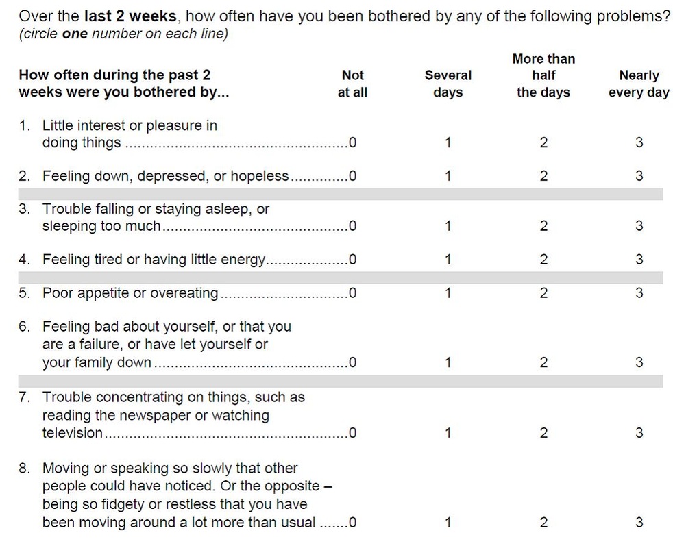
With the rise in easy access to social media and the internet, the psychological health of young adults and teenagers are prone to getting affected. Moreover, with the rise of the COVID-19, there has been an increase in depression and anxiety by 40% among the people. Neglecting to address this issue of mental health can lead to depression and in severe situations, even suicidal thoughts. Early detection of a quick and successful automated diagnosis of depression could be of great help. However, since a range of complicated symptoms is reported, this is an extremely difficult task. Depression causes cognitive and motor changes that affect speech production. Reduction in verbal activity productivity, prosodic speech irregularities, and monotonous speech have all been shown to be symptomatic of depression. The eight-item Patient Health Questionnaire depression scale (PHQ-8) has been used as a scale to classify the level of depression for the 189 participants from the DAIC-WOZ dataset. Each question was scored out of 3 and the total score was for 24. Based on previous research and experiments, a PHQ score greater than 10 depicted that the person suffered from depression.
Proposed Approach
In summary, the main contributions can be described as follows.
- First, deep learning models using GloVe word embeddings along with LSTMs, GRUs, TextCNNs, and BiLSTMs have been implemented.
- To draw attention to the important words used by depressed patients, BiLSTM with Attention Layer has been proposed.
- Second, due to the disadvantages of the context-independent nature of GloVe word embeddings, Embeddings of Language Model (ELMo), a context-dependent model has been used.
- Third, to understand the significance of transfer learning in 2NLP, Universal Language Model Fine Tuning (ULMFit) and Bidirectional Encoder Representation from Transformers (BERT) have been proposed for predicting the depression severity.
- Finally, a Python Flask Application using has been proposed which uses an ensemble method by averaging the predictions from all the algorithms that use GloVe word embeddings.
Dataset Used
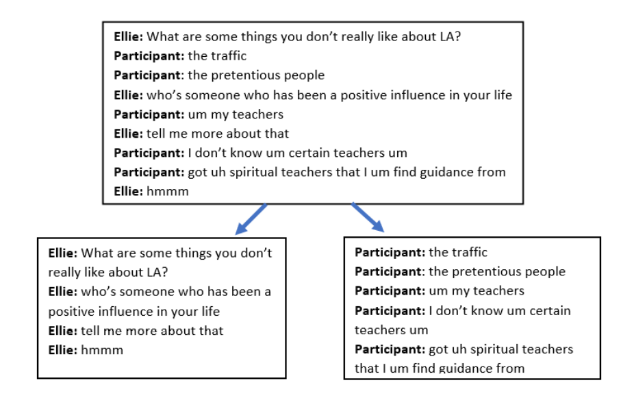
We have used the Distress Analysis Interview Corpus (DAIC-WOZ) dataset used in the Audio/Visual Emotion Challenge (AVEC 016). It includes text, audio, and video information of 189 interviews designed to enable the treatment of emotional disturbance, nervous breakdown and other mental health issues. We had seperated the questions and answers of the interview and particularly focussed on the answers given by the participants.
Preprocessing
The following steps have been used for pre-processing the data and producing tokenized words from the transcript file:
- Participant answers are subjected to stopword elimination and optionally stemming / lemmatization, and translated into a list of words.
- Word tokenization is done, after all the words used in the responses have been collected.
- By using a sliding window of size 10 the set of terms thus obtained is split into several sets.
- The corresponding tokens list is padded with zeros for lists (after windowing) that have less than 10 characters.
- For our layout, we use GloVe embedding, specifically embedding featuring 6 billion tokens, 400k word vocabulary and 100 dimensional vec8tors. A 2-D array is created which stores the vectors in the response vocabulary for each word (after removing the stopwords).

Feature selection and Extraction
Feature extraction had been carried out for the verbal responses of each participant as given in the transcript file. From previous research work, it has been noticed that there are changes in the prosodic tones in a depressed person than a normal person. Also, they speak for a lesser amount of time with longer pauses. Consequently, from the words spoken by the participantswhich was subsequently made into a transcribed format, the total words uttered by the participant is calculated, the average number of words has also been extracted in a similar manner. In addition, the time taken to complete the interview has also been taken into account. Furthermore, the count of the filler words such as “uh”,”um” etc. used by the participants has been calculated. The number of times the participant had uttered in terms of first person by using a lot of “I”s are counted. An analysis of the frequency of the number of positive and negative words such as hate, horrible, miserable etc. used by the participants has also been done. Harvard positive and negative word dictionary was used and the words used in the conversations were extracted the frequency of these words has also been found.
for filename in filenames:
    if filename.endswith('.csv'):
        #add participant id number to list
        participant_num.append(int(filename[:3]))
        #read in tab-delimited files
        df = pd.read_csv(filename, delimiter='\t')
        #drop unnecessary columns
        df.drop(['speaker'], axis=1, inplace=True)
        sentence_count = df.value.count()

        #whitespace tokenize
        tokens = df.value.apply(lambda x : tokenize(str(x)))
        total = len(tokens)
        total_words.append(total)

        average_words = total / sentence_count
    sentence_total.append(sentence_count)
    wps.append(average_words)
bins=[-1,0,5,10,15,25]
plt.figure()
plt.hist(ds_total["PHQ8_Score"], rwidth=0.6, bins=5)
plt.xlabel('PHQ8 score')
plt.ylabel('Number of participants')
plt.show()
plt.savefig('/content/drive/My Drive/Depression_detect/bins.png')
This graph provides an analysis of the PHQ-8 scores from the Patient Health Questionnaire (PHQ8) test to identify depression levels. The scores were treated from (0-25) in bins separating them into levels of depression: none (0), mild (0-5), moderate (5-10), moderately severe (10-15), severe (15- 25). The graph depicts that only a few cases show moderately severe and severe levels of depression.
pd.crosstab(ds_total.Gender, ds_total.level).plot(kind="bar", figsize=(10, 8), title="Gender");
plt.plot();
From the graph, it is clear that women are more prone to depression than men. ’0’ represents men and 1 represents women. (0-4) depicts the various levels of depression. Studies have shown that women are more prone to depression than men due to the hormonal variations that occur during puberty, postpartum depression and menopausal stages. Early recognition of depression due to such situations is necessary for maintaining are mentally healthier life.
Methodology
For text processing, there are three types of modelling approaches
- Context-free modelling uses any participant’s answer as an independent variable, with no information on the question or the time it was asked.
- Context-dependent modelling has a set of question-answer matching set,with a question and a corresponding answer
- Sequence modelling This modelling approach models reaction of the participant in a sequence and not based on a specific question.
GloVe Embeddings and BiLSTM model
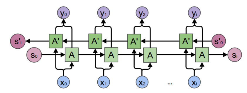
BiLSTMs have been used to take advantage of remembering information for long periods of time as well as understand the context in both the directions.They do so by providing a way to bring only relevant information from one stage to the next through various developments at the cell level such as forget gate, resetting gate, updating gate.In this model, we have used 2 LSTM layers, Adam optimizer and the categorical cross-entropy loss.
What are BiLSTMs?
Bidirectional Recurrent Neural networks have information about the sequence in both forward and backward manner ie. they are able to run inputs in two ways, one from past to future and one from future to past and what differs this approach from unidirectional is that in the LSTM that runs backward you preserve information from the future and using the two hidden states combined you are able in any point in time to preserve information from both past and future.
answer_inp = Input(shape=(windows_size, ))
embedding_size_glove = 100
answer_emb1 = Embedding(vocab_size_stop+1, embedding_size_glove, weights=[embedding_matrix_lp], input_length=windows_size, trainable=False)(answer_inp)


bi_lstm =  Bidirectional (LSTM (embedding_size_glove,return_sequences=True,dropout=0.50),merge_mode='concat')(answer_emb1)
model_bi1 = TimeDistributed(Dense(embedding_size_glove,activation='relu'))(bi_lstm) #TimeDistributed method is used to apply a Dense layer to each of the time-steps independently. We used Dropout and l2_reg regularizers to reduce overfitting.
model_bi2 = Flatten()(model_bi1)
model_bi3 = Dense(256,activation='relu')(model_bi2)
output = Dense(5,activation='softmax')(model_bi3)
model_bi = Model(answer_inp,output)
model_bi.compile(loss='categorical_crossentropy',optimizer='adam', metrics=['accuracy'])
model_bi.summary()
model_glove_bilstm = model_bi.fit(train_a_b, train_y_b, validation_data=(dev_a_b, dev_y_b), epochs=30, batch_size=64, shuffle=True, callbacks=[early_stopping])
GloVe Embeddings and CNN + LSTM (Hybrid Model)
A Hybrid Model consisting of CNN and LSTM has been used. Although LSTMs gave good results, it took a very long time to train the epochs. One way to speed up the training is to add a convolutional layer. CNNs pass a “filter” over the data and calculate a higher-level representation. In addition, LSTM can effectively retain historical information characteristics in long text sequences, and the local text characteristics are extracted using the CNN structure.
lstm_cnn = Sequential()
lstm_cnn.add(Embedding(vocab_size_stop+1, 100,weights=[embedding_matrix_lp],input_length=windows_size, trainable=False))
lstm_cnn.add(Conv1D(filters=32, kernel_size=3, padding='same', activation='relu')) #We can use a smallish set of 32 features with a small filter length of 3. The pooling layer can use the standard length of 2 to halve the feature map size.
lstm_cnn.add(MaxPooling1D(pool_size=2))
lstm_cnn.add(LSTM(100))
lstm_cnn.add(Dense(5, activation='softmax'))
lstm_cnn.compile(loss='categorical_crossentropy', optimizer='adam', metrics=['accuracy'])
## Fit train data
lstm_cnn.summary()
hist = lstm_cnn.fit(train_a_b, train_y_b, validation_data=(dev_a_b, dev_y_b), epochs=30, batch_size=64, shuffle=True, callbacks=[early_stopping])
GloVe Embeddings and BiLSTM with Attention Layer
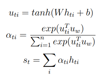
The further updates were made to the same BiLSTM function. The BiLSTM sums up the information from both the left and right directions. The self-attention layer tries to capture the more important parts of a sentence when different aspect-terms are input. BiLSTM model followed by Attention layer with adam optimizer and softmax activation has been used. This proposed model uses contextual knowledge and semantic features effectively, and in particular model correlations between aspect-terms and context words. Rather than paying attention to individual input vectors of the input sequence based on the attention weights, the basic concept of using Attention Mechanism is to avoid attempting to learn a single vector representation for each sentence.
class AttentionLayer(Layer):
    """
    Attention operation, with a context/query vector, for temporal data.
    Supports Masking.
    Follows the work of Yang et al. [https://www.cs.cmu.edu/~diyiy/docs/naacl16.pdf]
    "Hierarchical Attention Networks for Document Classification"
    by using a context vector to assist the attention
    # Input shape
        3D tensor with shape: `(samples, steps, features)`.
    # Output shape
        2D tensor with shape: `(samples, features)`.
    How to use:
    Just put it on top of an RNN Layer (GRU/LSTM/SimpleRNN) with return_sequences=True.
    The dimensions are inferred based on the output shape of the RNN.
    Note: The layer has been tested with Keras 2.0.6
    Example:
        model.add(LSTM(64, return_sequences=True))
        model.add(AttentionWithContext())
        # next add a Dense layer (for classification/regression) or whatever...
    """
    def __init__(self, **kwargs):
        self.init = initializers.get('glorot_uniform')
        super(AttentionLayer, self).__init__(**kwargs)

    def build(self, input_shape):
        assert len(input_shape) == 3

        self.W = self.add_weight(name='Attention_Weight',
                                 shape=(input_shape[-1], input_shape[-1]),
                                 initializer=self.init,
                                 trainable=True)
        self.b = self.add_weight(name='Attention_Bias',
                                 shape=(input_shape[-1], ),
                                 initializer=self.init,
                                 trainable=True)
        self.u = self.add_weight(name='Attention_Context_Vector',
                                 shape=(input_shape[-1], 1),
                                 initializer=self.init,
                                 trainable=True)
        super(AttentionLayer, self).build(input_shape)

    def compute_mask(self, input, input_mask=None):
        # do not pass the mask to the next layers
        return None

    def call(self, x):
        # refer to the original paper
        # link: https://www.cs.cmu.edu/~hovy/papers/16HLT-hierarchical-attention-networks.pdf

        u_it = K.tanh(K.dot(x, self.W) + self.b)

       #Through structure the vector applied  is used as
        #Make attention value into probability distribution through
        a_it = K.dot(u_it, self.u)
        a_it = K.squeeze(a_it, -1)
        a_it = K.softmax(a_it)

        return a_it

    def compute_output_shape(self, input_shape):
        return (input_shape[0], input_shape[1])
lstm_dim=50
bilstm = Bidirectional(LSTM(lstm_dim, return_sequences=True))(answer_emb1)  #Input should be three dimensional
# bilstm = LSTM(2*lstm_dim, return_sequences=True)(input_data)
# bilstm_output = Dense(1)(bilstm)

attention_layer = AttentionLayer()(bilstm)
print(attention_layer)
repeated_word_attention = RepeatVector(lstm_dim * 2)(attention_layer)
repeated_word_attention = Permute([2, 1])(repeated_word_attention)
sentence_representation = Multiply()([bilstm, repeated_word_attention])
sentence_representation = Lambda(lambda x: K.sum(x, axis=1))(sentence_representation) #total summation of the multiplied bilstm and attention

bilstm_output = Dense(5,activation='softmax')(sentence_representation)

model = Model(inputs=[answer_inp],
            outputs=[bilstm_output])
model.compile(loss='categorical_crossentropy', optimizer='adam',metrics=['accuracy'])
model.summary()
Transfer Learning
The ability to transfer knowledge from a pre-trained model to a new model is called Transfer Learning. Language modeling is transfer learning in the field of NLP. It is the task of predicting the next word in a sequence. In addition, language modeling has the desirable property of not requiring labeled training data. Raw text is abundantly available for every conceivable domain. These two properties make language modeling an ideal fit for learning generalizable base models.
Here we will explore on: ELMo, ULMFiT and BERT.
Embeddings of Language Models (ELMo)
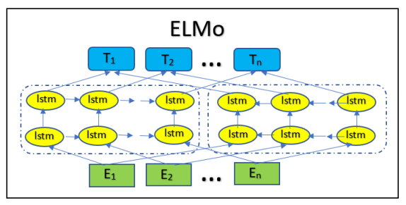
Due to the disadvantages faced by the context independent nature of GloVe embeddings, ELMo embeddings has been incorporated. ELMo is a deep contextualized representation of words that models both dynamic word utilization features, and the variations in semantic understandings. Developed by Allen NLP, the state-of-art pretrained model is context dependent. ELMo uses two bidirectional LSTMs in training, so the language paradigm knows both the succeeding and the preceeding words in the expression fed to the model. This consists of a two-layer, bidirectional LSTM backbone. ELMo pre-trained on the 1 trillion Word Benchmark, is a character based word embeddings allowing the network to use morphological features of the words to form representation for out-of-word vocabulary tokens unseen during training.
def elmo_vectors(x):
  embeddings = elmo(x.tolist(), signature="default", as_dict=True)["elmo"]

  with tf.Session() as sess:
    sess.run(tf.global_variables_initializer())
    sess.run(tf.tables_initializer())
    # return average of ELMo features
    return sess.run(tf.reduce_mean(embeddings,1))
Universal Language Model-Fine Tuning (ULMFiT)
ULMFiT works using the concept of inductive transfer learning. Inductive
transfer refers to a learning mechanism’s ability to improve performance on the present task after learning a different but related concept or skill on a prior task. Language model pretrained on the WikiText-103 dataset has been used to train the target task which is then fine tuned for the classification model. In the proposed approach, the pre-trained language model is fine tuned on the target DAIC-WOZ dataset. A classifier is then used on the fine-tuned data to classify the texts based on the levels of depression.
Bidirectional Encoder Representations of Transformers (BERT)
In the RNNs tried earlier and even those tried with attention are all sequential. Tasks cannot be carried out parallely .This lack of parallelization within a series can not be compensated either by adding more samples in a training batch, as loading and optimizing weights for different samples increases memory requirements which will thereby limit the number of samples that can be included in a batch. Solving some of these issues lead to explore the Transformer model. The model BERT is chosen because it encompasses Transformers in it’s architecture and has been a proven benchmark in Natural Language Processing.
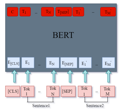
BERT is a trained stack of Transformer Encoders. Both sizes of the BERT model have a large number of encoder layers-twelve for the Base version, and twenty-four for the Large. We also have bigger feed-forward networks (768 and 1024 hidden units respectively), and more headers of attention (12 and 16 respectively) than the default configuration in the Transformer reference implementation (6 encoder layers, 512 hidden units and 8 headers of attention).The first input token has a special [CLS] token attached to it. CLS stands for Classification here. BERT takes as its input a sequence of words that keep flowing up the stack. Each layer applies self-attention, passes the results through a feed-forward network, then hands it over to the encoder that follows. As far as architecture is concerned, everything has so far been the same as the Transformer (aside from scale, which are only configurations we must set). It is at the output that we begin to see how things diverge first. Each location gives out a hidden size vector (768 in BERT Base). The vector can now be used since we choose the input for a classifier
from keras.regularizers import l2
def build_model(bert_layer, max_len=512):
    input_word_ids = Input(shape=(max_len,), dtype=tf.int32, name="input_word_ids")
    input_mask = Input(shape=(max_len,), dtype=tf.int32, name="input_mask")
    segment_ids = Input(shape=(max_len,), dtype=tf.int32, name="segment_ids")

    _, sequence_output = bert_layer([input_word_ids, input_mask, segment_ids])
    clf_output = sequence_output[:, 0, :]
    hidden1=Dense(64, kernel_regularizer=l2(0.03), bias_regularizer=l2(0.03) ,activation='relu')(clf_output)
    out = Dense(5 ,activation='softmax')(hidden1)

    model = Model(inputs=[input_word_ids, input_mask, segment_ids], outputs=out)
    model.compile(Adam(lr=2e-6), loss='categorical_crossentropy', metrics=['accuracy'])

    return model
Results
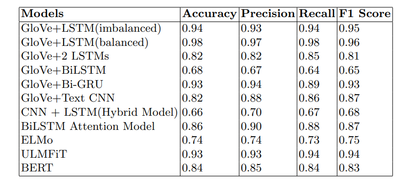
After running 30 epochs for the GloVe word embeddings + LSTM model with Adam optimization and categorical cross entropy loss, a test accuracy of 94.7% was obtained without balancing the dataset. After the balancing the dataset, the accuracy increased to 98.6% with a test loss of 4.3%. Due to the significance of context dependency in sentences, ELMo was incorporated and gave an accuracy of 73.1%. Experimental results showed that the model with balanced data worked better than the imbalanced data. After implementing transfer learning using ULMFiT and BERT, it was observed that both the models performed well by obtaining an accuracy of 93.2% and BERT model with 84%
from flask import Flask
app = Flask(__name__,static_url_path='/static')
run_with_ngrok(app)   #starts ngrok when the app is run
@app.route('/')
def home():
    return render_template("index.html")
    #return "<h1>Running Flask!</h1>"

@app.route('/predict', methods=['GET','POST'])

if __name__ == "__main__":
    app.run()
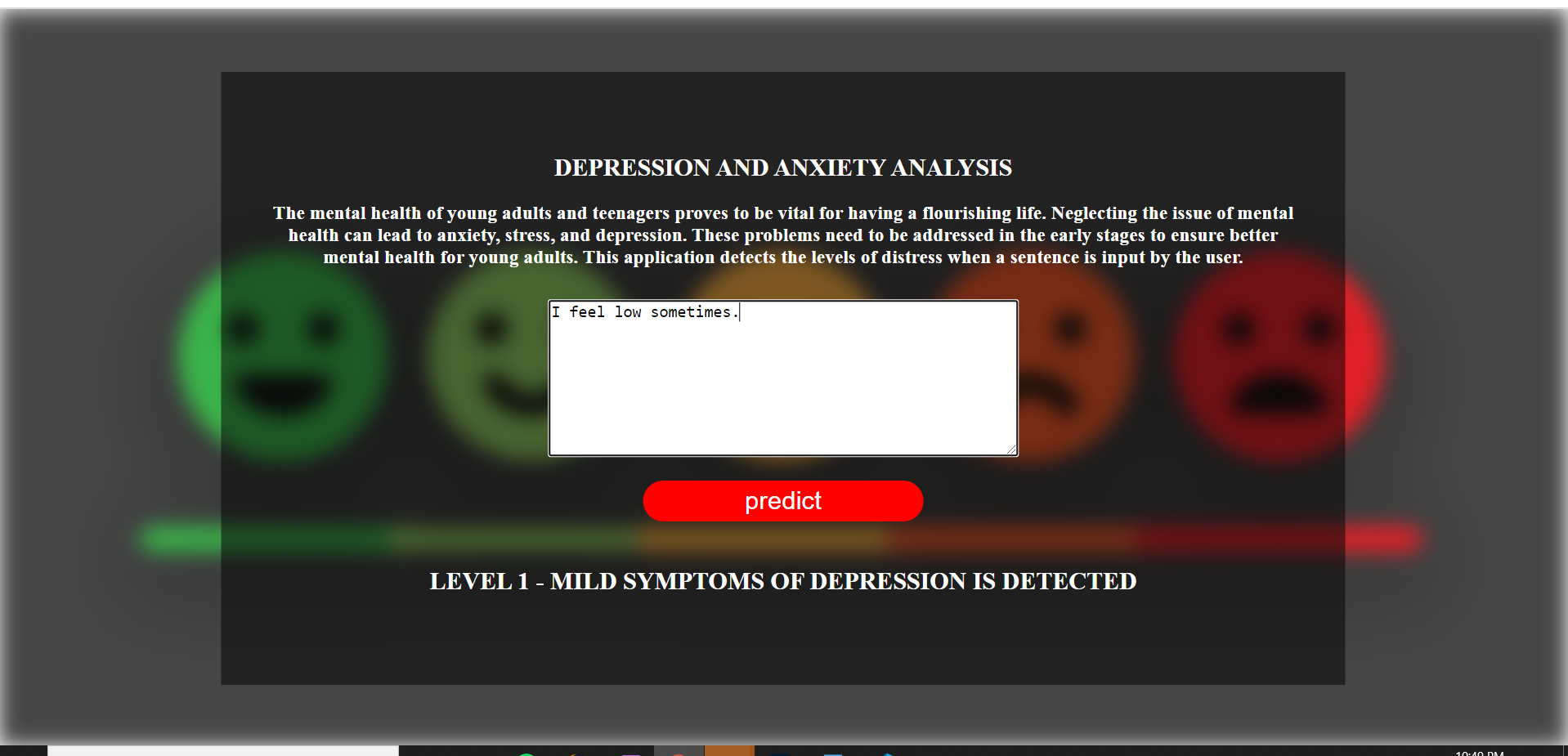
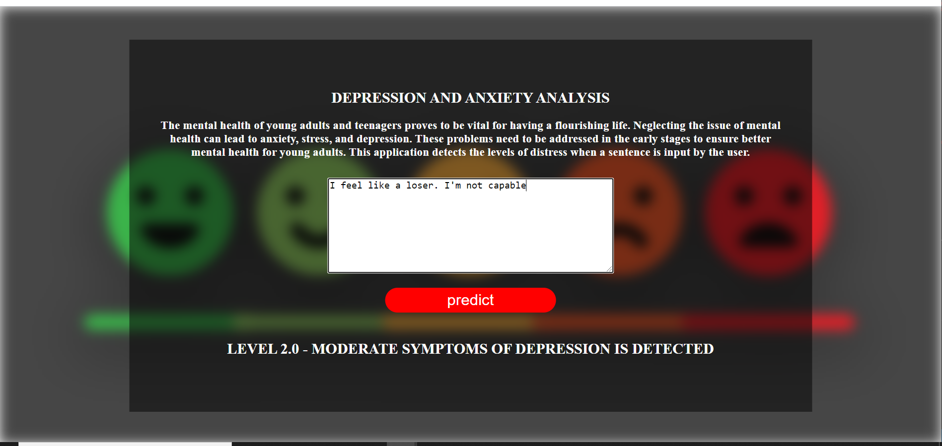
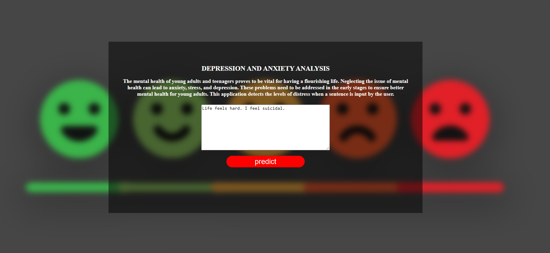
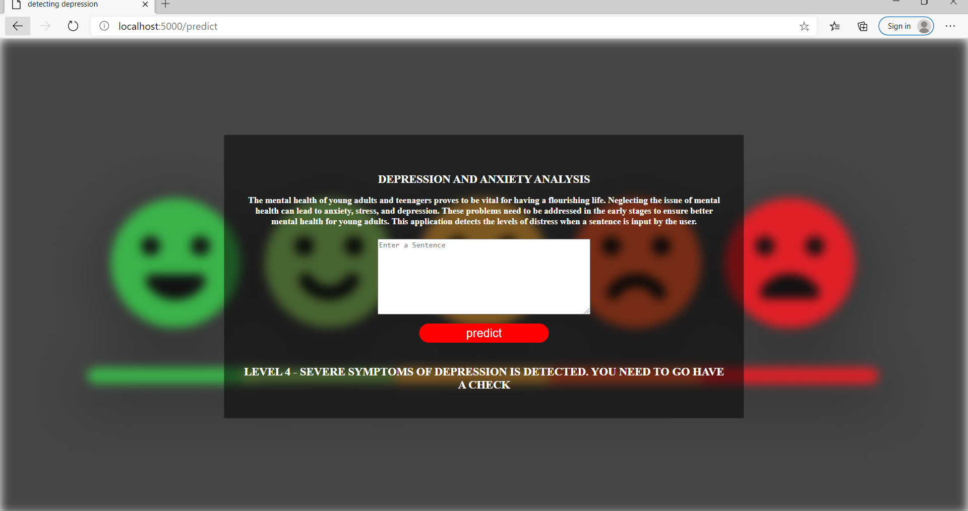
Here are some snippets of the Flask Application that I had deployes using the glove embeddings and LSTM model.
Conclusion
The objective of detecting depression through textual information involved in understanding the verbal and sentimental usage of words by the participants. Experimental results showed that the model with the balanced data worked better than the imbalanced data. The BERT model gave good results and the GloVe+LSTM model outperformed all other models. Moreover, work needs to be done to explore Explainable AI in order to understand decision making processes in the mild/severe levels which will help in understanding the models better because understanding the output is pivotal for researchers and professionals alike. Since the scope of the project has been. restricted to textual information, the scope of the project can be widened to explore on the analysis of audio and video features using deep learning techniques. Furthermore, detecting depression on social media such as Facebook or twitter can also be done in the future.
References
[1] Fabien Ringeval, Bj¨orn Schuller, Michel Valstar, Jonathan Gratch, Roddy Cowie, et al.. AVEC 2017 - -”Life Depression, and Affect Recognition Workshop and Challenge”. 7th International Workshop on Audio/Visual Emotion Challenge, AVEC’17, co-located with the 25th ACM International Conference on Multimedia, MM, Oct 2017, Mountain View, United States. pp.3-9
[2] https://github.com/kykiefer/depression-detect
[3] Syed Arbaaz Qureshi, Mohammed Hasanuzzaman, Sriparna Saha Gael Dias -”The Verbal and Non Verbal Signals of Depression - Combining Acoustics,Text and Visuals for Estimating Depression Level”IEEE 2019
[4] Ashwath Kumar Salimath,Robin K Thomas,Sethuram Ramalinga Reddy ”Detecting Levels of Depression in Text Based on Metrics”(arXiv:1807.03397v1 2018)
[5] Yang, Le ’I&’ Sahli, Hichem ’I&’ Xia, Xiaohan ’I&’ Pei, Ercheng ’I&’ Oveneke, Meshia Jiang, Dongmei. Hybrid Depression Classification and Estimation from Audio Video and Text Information” 45-51. 10.1145/3133944.3133950
[6] Thanapapas Horsuwan1 , Kasidis Kanwatchara1 , Peerapon Vateekul1 , and Boonserm Kijsirikul1 “A Comparative Study of Pretrained Language Models on Thai Social Text Categorization “- arXiv:1912.01580 (2019)
[7] https://towardsdatascience.com/transfer-learning-in-nlp-fecc59f546e4
